Machine Learning Model for Identifying Cancer in Brain MRIs

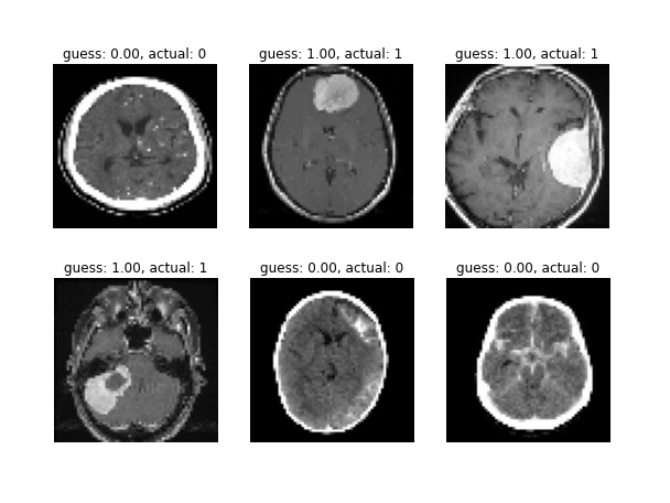
In 11th grade, I coded a Convolutional Neural Network in Python (using the Keras framework) that tries to identify meningiomas in brain MRIs. It ended up with more than 99% accuracy on the testing set. The image below shows a random sample of the testing set along with the neural network's guesses.

I found the dataset of brain MRI scans on a website called Kaggle and the dataset has two categories: training images and testing images. It has a total of 1217 training images and 220 testing images labeled either "no tumor" or "meningioma tumor".

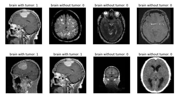
The Python script begins by preprocessing the input data. Using the Keras library, the script resizes the images, which come in many shapes and sizes, into 64 × 64-pixel grayscale squares. Then, it loads these images into arrays for the training and testing sets while keeping track of the images' labels. Rather than using string labels, the script quantifies the English diagnoses by labeling healthy brains with a 0 and meningioma-containing brains with a 1. Below is a sample of eight labeled images after preprocessing.

The model begins with a single 64 × 64 image as the input layer. The next layer convolves the image with 32 filters, resulting in 32 new 64 × 64 images. The filters are 3 × 3 images whose pixel values are parameters of the model, and each filter's convolution of the input image may reveal different features of the brain MRI scan. The next layer compresses the 32 images by reducing each 2 × 2-pixel square into a single pixel through max-pooling where the value of each resultant pixel is the maximum of the values of its four predecessors. Max-pooling is preferable to simply averaging because it ensures that relevant features are "noticed" and passed on to the next layer. After the first max-pooling layer, each image is 32 × 32 pixels. The model repeats the convolution and max-pooling layers until the images are each 4 × 4 pixels wide.

At this point, the images are too small for convolution with a 3 × 3 filter to be intuitive, so the model "flattens" the layer by unraveling the images into a one-dimensional array of 512 neurons. Next is a typical "dense" layer whose 256 neurons each provide a weighted sum of the values of the 512 neurons in the previous layer. The "dropout" layer in between randomly zeroes about half of those 512 neurons' values, which deters the model from over-fitting the training data or relying heavily on only a few neurons. Finally, the last layer consists of a single neuron that computes a weighted sum of the previous layer to provide a diagnosis in the form of a number between 0 and 1, where a 1 indicates the presence of a meningioma and a 0 indicates the lack thereof.

After training the model for 15 epochs, it reached an accuracy of 99.55% on the testing dataset.

See this project's Python notebook and its accompanying dataset on Kaggle ↗.